In a previous blog post and video, we showed how to use Tableau to create maps of a tag’s location history. In this post, we will use Tableau maps to show how WISER Systems tunes some of the tracking settings of a mesh to the particulars of the site where it is installed. Your WISER support representative will take care of this initial setup work, so here is just a peek behind the curtain of how we adapt the data pipeline for different installations.
We have a tracking mesh running in our office which I intentionally sabotaged to create some areas that track poorly. I then walked around with a tag in each hand. In the plot below, you can see our office floorplan, with a blue dot for every tracked location of my right hand, and orange dots for my left hand. On the left side, it looks as if we are tracking outside of the building (untrue), and on the right side, a lot of points are missing. Sabotage successful. Let’s look at what’s going on here.
Each tag in the mesh will “ping,” broadcast a message at a periodic interval. Each ping is collected by the Antennas in the mesh and turned into a location with X and Y coordinates by the server. That location is based on measurements, and it will have some statistical variation from the “true” location.
These are “raw” locations before being post-processed. What a mess! But even now, in the center of our office you can see precise trails where tracking was quite good.
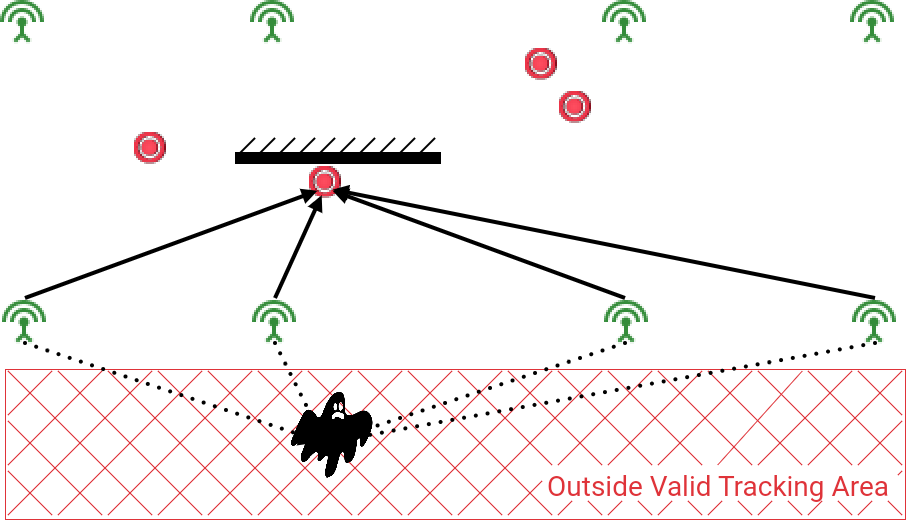
We can then apply some basic processing to improve the reported location. First, we exclude outliers. One method is to set a “Valid Tracking Area” geofence. For example, if we know a tag will never be outside of a building, any measurement there is erroneous. One way this can happen is with a tag that is partially obstructed along the edge of a mesh. If Antennas on the inside of the mesh are blocked, and the Antennas on the edge have been installed in a straight line, then the first “ping” received from a tag could be on either side of the line of Antennas, either the right location or the location of its reflection. The defined Valid Tracking Area eliminates the reflection ghost.
Next, as part of the location calculation, the algorithm assigns an error value to the result. We can set a threshold to throw out measurements where the error is too large. In environments that are cluttered and noisy in radiofrequency, we may need to accept measurements with larger errors.
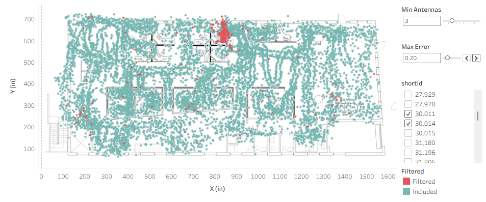
If I slice our raw locations by error, you can see my desk! When the tags are sitting on my desk, partially obstructed, tracking is sometimes poor.
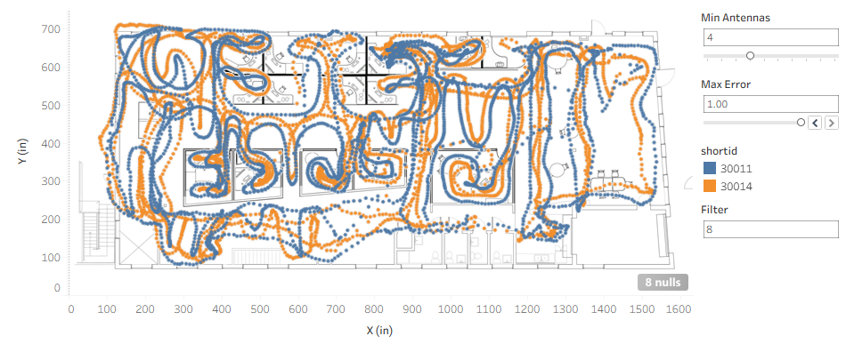
Next, we set a threshold for the minimum number of Antennas that need to have participated in a location calculation. The more Antennas, the higher the confidence. If the highest accuracy is not needed, sites can spread Antennas farther apart, and fewer Antennas will participate in each location. For some applications, it is sufficient to know a tag is inside the building, while in others, the location needs to be known within 6″ accuracy.
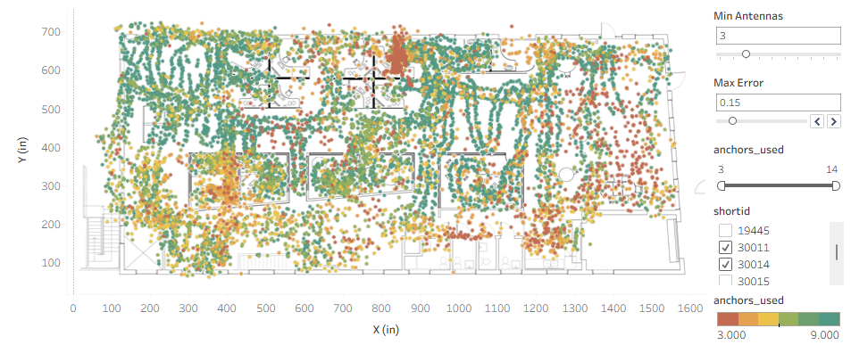
Coloring our raw locations by number of Antennas, we see the right side of the office does not have sufficient Antenna coverage for high accuracy.
With the outliers removed, we then average the last few data points to remove statistical noise. There is a tradeoff between precision and latency. At a lower filtering value of 2 or 4, the reported location will track the actual location almost in real-time, but with much more jitter. At 4 or more, even up to 20 or 30 or more, more samples are used to calculate the location, with the caveat that the reported position will tend to lag behind the actual position if the tag is moving. If a stationary tag is pinging only once a minute, and we’re averaging roughly 30 samples, we may be tracking 15 minutes or more in the past. This is OK if we just want to find a tag 12 months from now, but can become a problem for workflow analytics or triggering automations with geofences.
In practice, we “filter” locations by applying an exponential moving average (EMA), which gives more weight to recent samples and exponentially less weight to older ones. The filter value we specify is the inverse of alpha, the span, which is effectively the number of location samples to include in the average.
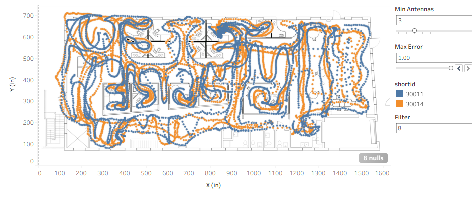
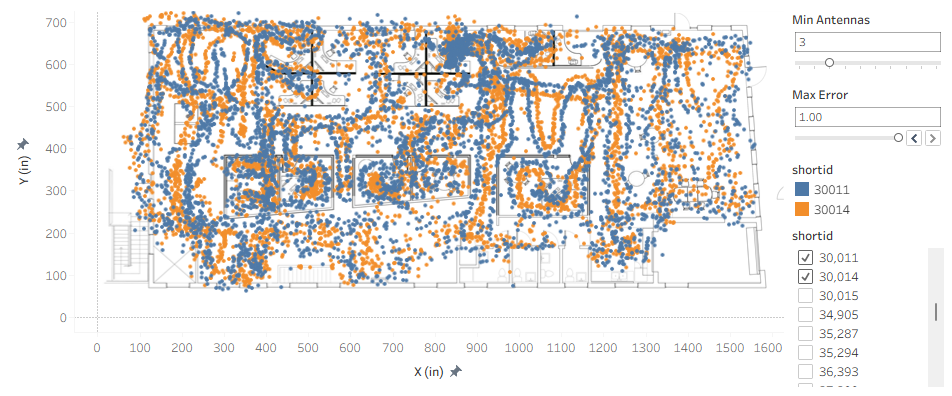
Here is that averaged data without any thresholds applied, and you can see more points are recorded on the right side of the building, where fewer Antennas received the tags’ pings.
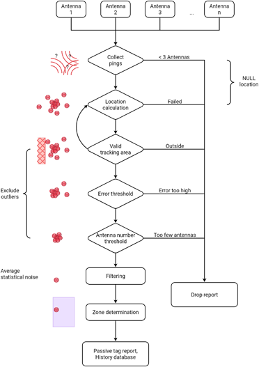
Here is a flow chart of the entire processing pipeline.
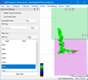
We can compare the location reported by a stationary tag over a long period of time with and without this pipeline enabled. You can see how the reported location is compressed to an accurate point. We can do similar for a tag moving along a known path. I can’t show you the time lag in a blog post, but if I move the tag along the corner of a desk on a right angle, you can see how the higher filtering smooths out the corner.
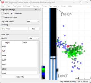
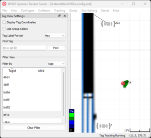
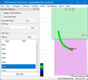
Caption: History visualization in the server to help with tuning. The processed location is precise to under 6 inches!
And what was going on at the left side of the office? An Antenna has been moved, so the initial automatic calibration no longer matches reality. It is sometimes possible to successfully track with Antennas in the wrong location, and even though the statistics are good, it is obviously not ideal. We want to correct the antenna problem as soon as possible to get good quality location data. For that, we have a separate diagnostic system, the Mesh Monitor, to alert on these kinds of issues. We will cover that in a later blog post.
Before setting up a site, your WISER support representative will ask about the desired accuracy, the density of equipment and other obstructions, as well as whether the location data is needed in transit or just at rest. Then once the system is installed, all of these tracking settings knobs are adjusted so that location tracking is appropriate for the site and application. This is how we work with our customers to get you the best possible accuracy for a long time.
If you are interested in talking with someone from WISER about how we can help at your facility, please feel free to reach out. You can contact us via our website, email, or phone.